知乎原文
一些关于梯度累加的常见错误认识
代码
关于梯度累加的pytorch实现中,在网上查到的常见步骤如下:
for i, (context, label) in enumerate(train_loader):
    pred = model(context) #前向过程
    loss = loss_func(pred, label) #计算loss

    loss = loss / accumulation_steps  #为什么会有这个步骤?
    loss.backward() #求解梯度,注意此步骤只求了梯度,并没有将梯度更新

    if (i + 1) % accumulation_steps == 0: #只有当累积到accumulation_steps整数倍的时候
        optimizer.step()  #梯度才会更新
        optimizer.zero_grad()  #梯度清零
其中代码中的疑问步骤是:loss = loss / accumulation_steps,这一步是否需要?网上鲜有内容说清楚了这个细节。甚至还有不少错误的文章把该步骤写成loss += loss / accumulation_steps,这是错误的写法。
首先解释为什么要引入梯度累加。比如batchsize=100可以达到最优的优化结果,但是限于显卡的性能,batchsize=100会爆显存。我希望能够以batchsize=100的跑模型而不爆显存,一个解决方案是设置batchsize=50,即一个step有50个数据。但并不是每个step都更新梯度,而是每个偶数step更新梯度,这样可以达到几乎等价于batchsize=100的效果。
以loss函数为mse函数为例,梯度更新的公式是 $w=w-l\cdot\frac{\partial loss}{\partial w}\\=w-l\cdot\frac{\partial \sum_{i=1}^{100}{(ypred-ytrue)^2}}{\partial w}\\=w-(l\cdot\frac{\partial \sum_{i=1}^{50}{(ypred-ytrue)^2}}{\partial w}+l\cdot\frac{\partial \sum_{i=51}^{100}{(ypred-ytrue)^2}}{\partial w})\\=w-l\cdot(\frac{\partial loss1}{\partial w}+\frac{\partial loss2}{\partial w})$
直接计算 会爆显存,于是改为先计算前50个数据的 ,再计算后50个数据的 ,两个梯度加起来,等价于一起计算100个数据的 。
由于loss.backward()是自动累加梯度的,只要没有手动将梯度清零,它会基于之前的梯度累加。因此不需要做额外的操作。loss = loss / accumulation_steps这一步是额外的操作。
但如果loss的定义不是 ,而是
那么 $w=w-l\cdot\frac{\partial loss}{\partial w}\\=w-l\cdot\frac{1}{100}\cdot\frac{\partial \sum_{i=1}^{100}{(ypred-ytrue)^2}}{\partial w}\\=w-(l\cdot\frac{1}{100}\frac{\partial \sum_{i=1}^{50}{(ypred-ytrue)^2}}{\partial w}+l\cdot\frac{1}{100}\frac{\partial \sum_{i=51}^{100}{(ypred-ytrue)^2}}{\partial w})\\=w-l\cdot(\frac{1}{2}\frac{\partial loss1}{\partial w}+\frac{1}{2}\frac{\partial loss2}{\partial w})$
如果每个小批的大小一样,而且凑满了一组,那就把每个小批的平均 loss 除以累加步数。
也就是说,是否需要loss = loss / accumulation_steps这个步骤取决于对loss的定义,如果loss的定义是整个batch内求和,则不需要加上该步骤。
另一个错误的写法
一个思考,上面说到loss += loss / accumulation_steps 是错误的写法,但如果将求梯度的步骤挪出去,如下面的代码所示,是否正确了?问题出在哪里?
# 初始化total_loss为0
total_loss = torch.zeros(1).to(device)
optimizer.zero_grad()  # 在起始时清零梯度

for i, (context, label) in enumerate(train_loader):
    context = context.to(device)
    label = label.to(device)
    pred = model(context)  # 前向过程
    loss = loss_func(pred, label)  # 计算损失

    # 累积损失,除以accumulation_steps以便模仿较大批量大小的梯度
    total_loss += loss / accumulation_steps

    # 一旦累积了足够的步数,反向传播梯度
    if (i + 1) % accumulation_steps == 0:
        total_loss.backward()  # 对累积的总损失求梯度
        optimizer.step()  # 进行梯度更新
        optimizer.zero_grad()  # 清空累积梯度
        # 重新初始化total_loss为0,为下一个累积步骤做准备
        total_loss = torch.zeros(1).to(device)

# 注意:在循环结束后检查是否需要处理剩余梯度
if total_loss.item() != 0:
    total_loss.backward()
    optimizer.step()
    optimizer.zero_grad()
202406更新:
几个小批的 loss 可以先加起来,最后一起反传。只是这样一来,每个小批前向时留下的中间结果都得留到最后,更占显存。为什么要留?因为反向传播算梯度时,还要用到前向算出来的激活值。
下面的代码可以说明在反向传播的过程中,激活值是必不可少的部分。
import torch

# 设定随机种子以保证结果的可复现性
torch.manual_seed(0)

# 假设这是我们的激活值矩阵a,形状为[10, 1]
a = torch.randn(10, 1, requires_grad=True)

# 这是权重w,形状为[1, 1]
w = torch.randn(1, 1, requires_grad=True)

# 计算模型的输出y
y = a * w

# 假设我们有一个目标值t,这里我们使用一个全1的向量作为示例
t = torch.ones(10, 1)
y.retain_grad()

# 计算损失值,这里使用均方误差作为损失函数
loss = (y - t).pow(2).mean()

# 反向传播,计算梯度
loss.backward()

print('a',a)
print('loss',loss)
print('y.grad',y.grad)
# 打印权重w的梯度
print("梯度相对于权重w:", w.grad)
在这个例子中,y=w*a,loss=(y-1)^2
其中a的shape是[10,1],表明一个batchsize内有10个不同的数据。w是标量,表示这个神经网络只有一个参数。那么y的shape也是[10,1]。
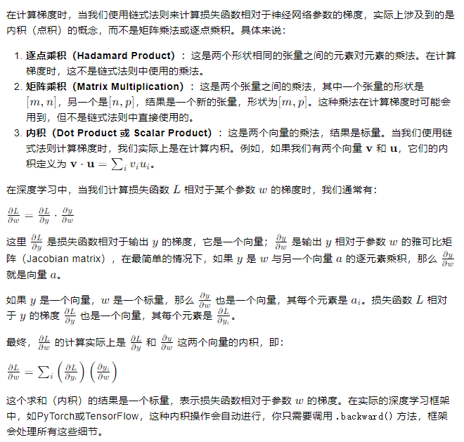
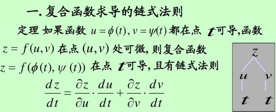
根据链式法则,∂loss/∂w=(∂loss/∂y)*(∂y/∂w)=(∂loss/∂y)*a
其中∂loss/∂y就是y.grad
你会发现,y.grad和a的内积就是w.grad
也就是说,在计算w.grad的时候,是需要用到a是整个批次的所有的值的。
这里有一个小细节,y.grad的shape是torch.Size([10, 1]),a的shape也是torch.Size([10, 1]),两者如何相乘?这其实是逐点相乘然后相加得出最终的结果,最终的结果是w的梯度,它是一个标量。相当于做一个内积。
用代码验证梯度累积的等价性
梯度累积指的是在累积到一定steps后再做梯度更新的操作,此操作在一般情况下和直接用大batch是等价的。
我想验证这种等价性,即,情况1:不使用梯度累积,batchsize=b1
情况2:使用梯度累积,batchsize = b1/accumulation_steps
两种情况的训练成果是否等价?
直接上代码:
import torch
import torch.nn as nn
import torch.optim as optim
from torch.utils.data import TensorDataset, DataLoader

# Step 1: 创建数据集
# 假设我们有以下的数据(输入x和输出y),数据量为6
x_data = torch.tensor([[1.0], [2.0], [3.0], [4.0], [5.0], [6.0]])
y_data = torch.tensor([[2.0], [4.0], [6.0], [8.0], [10.0], [12.0]])

# 创建一个 TensorDataset 和 DataLoader
dataset = TensorDataset(x_data, y_data)
batch_size = 2
dataloader = DataLoader(dataset, batch_size=batch_size, shuffle=False)

# Step 2: 定义模型
class LinearModel(nn.Module):
    def __init__(self):
        super(LinearModel, self).__init__()
        self.linear = nn.Linear(1, 1)
        # self.bn = nn.BatchNorm1d(1)

    def forward(self, x):
        x = self.linear(x)
        # x = self.bn(x)
        return x

model = LinearModel()
model.train()

# 指定初始参数
with torch.no_grad():
    model.linear.weight.fill_(0.5)  # 设定权重初始值为0.5
    model.linear.bias.fill_(-1.0)   # 设定偏差初始值为-1.0

# Step 3: 定义损失函数和优化器
criterion = nn.MSELoss()
optimizer = optim.SGD(model.parameters(), lr=0.01)

# Step 4: 训练模型
epochs = 2
accumulation_steps = 2  # 设置梯度累积步数(在这个例子中每个epoch训练3次)

for epoch in range(epochs):
    optimizer.zero_grad()  # 清空梯度
    accumulated_loss = 0.0
    # accumulated_loss.requires_grad=True

    # 使用 DataLoader 迭代数据
    for i, (inputs, targets) in enumerate(dataloader):
        y_pred = model(inputs)
        # print('===epoch:{}  batch:{}'.format(epoch,i),'\n',
        #       'y_pred:',[[round(num, 2) for num in sublist] for sublist in y_pred.tolist()],'\n',
        #       'targets:',[[round(num, 2) for num in sublist] for sublist in targets.tolist()],'\n',
        #       'inputs:',[[round(num, 2) for num in sublist] for sublist in inputs.tolist()]
        #       )
        loss = criterion(y_pred, targets)
        loss = loss / accumulation_steps
        # print('loss:',loss.tolist())
        loss.backward()  # 反向传播,但不立即更新权重
        # print(f'linear Weight Grad: {model.linear.weight.grad}, Bias Grad: {model.linear.bias.grad}')
        # print(f'bn Weight Grad: {model.bn.weight.grad}, Bias Grad: {model.bn.bias.grad}')
        accumulated_loss += loss.item()

        # 每 `accumulation_steps` 步后更新权重
        if (i + 1) % accumulation_steps == 0 or (i + 1) == len(dataloader):
            # accumulated_loss.backward()
            optimizer.step()
            optimizer.zero_grad()

    # print(f'Epoch: {epoch+1}/{epochs}, accumulated_loss: {accumulated_loss / len(dataloader)}')

print("Training finished")
print('accumulation_steps:',accumulation_steps,' batch_size:',batch_size)
print('model.linear.weight',model.linear.weight)
print('model.linear.bias',model.linear.bias)
# print('model.bn.weight',model.bn.weight)
# print('model.bn.bias',model.bn.bias)
以下是我做了几次实验的结果:
Training finished
accumulation_steps: 2  batch_size: 3
model.linear.weight Parameter containing:
tensor([[1.3820]], requires_grad=True)
model.linear.bias Parameter containing:
tensor([-0.7893], requires_grad=True)

Training finished
accumulation_steps: 3  batch_size: 2
model.linear.weight Parameter containing:
tensor([[1.3820]], requires_grad=True)
model.linear.bias Parameter containing:
tensor([-0.7893], requires_grad=True)

Training finished
accumulation_steps: 1  batch_size: 6
model.linear.weight Parameter containing:
tensor([[1.3820]], requires_grad=True)
model.linear.bias Parameter containing:
tensor([-0.7893], requires_grad=True)

Training finished
accumulation_steps: 6  batch_size: 1
model.linear.weight Parameter containing:
tensor([[1.3820]], requires_grad=True)
model.linear.bias Parameter containing:
tensor([-0.7893], requires_grad=True)

Training finished
accumulation_steps: 2  batch_size: 2
model.linear.weight Parameter containing:
tensor([[1.5977]], requires_grad=True)
model.linear.bias Parameter containing:
tensor([-0.7290], requires_grad=True)
可以看到,前四种设定每次都用同样的 6 个样本更新,最后得到了同样的参数。最后一种设定每轮先用 4 个样本更新,再用剩下的 2 个更新。第二次只剩一个小批,代码还把它的平均 loss 除以 2,梯度就只有本来的一半。上面这组数字是按原代码得到的。
有几个细节需要注意。
(1)可以打乱数据。比较这两种写法时,只要每次拿来更新的样本是同一组,各组的更新顺序也一样。
(2)这里的 accumulated_loss 加的是 loss.item() 取出来的普通数字,只能用来记数,不能反传。如果加的是 loss 张量本身,哪怕它只有一个值,也可以反传。
(3)训练时,BN 用的是眼前这批数据的均值和方差。把一大批拆成几小批,这两个数就可能变,所以算出来的梯度也可能不一样。BN 本身不把输出限制在 0 到 1。